ds.cd <- readRDS("data/CellDeath.obj")3 Let’s get the hands dirty
Enough talked. How would we apply all this in practice?
3.1 Data set : Cell infections
The first data set is obtained in an experiment on infection of cell cultures by virus particles.
If you wish to try it yourself: you can find the data set CellDeath.obj here.
Store it on you computer and load it like this (after adapting to your path)
Cell cultures are brought in-vitro in contact with a virus. After some time the scientist checks in which cultures cell death is found.
There are six variations of cell cultures and infection methods: reference and T1 to T5. The details about the treatments are for the time being not important.
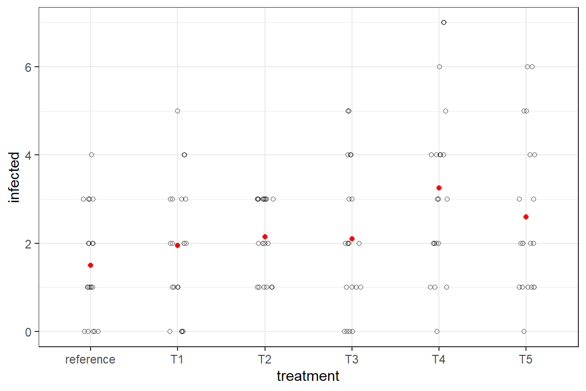
For each variation, four 12-well plates are entirely filled with the cell cultures and all cells are infected. Hence, one run of the experiment consists of 4 x 6 plates and five such runs are started. Per treatment, this leads to 20 counts confined between 0 and 12.
The result are stored in dataset ds.cd is shown in the graph below. The discrete nature is clearly visible. The red dots are a naive mean of the counts.
The reference method is least infected, yet all treatments have plates where none of the wells show infection.
The data set has at the same time an issue with dependence (observations grouped in runs and wells) and is clearly not normal distributed. In the previous paragraph we learned that proportions obtained via counts on a small and known total (12 wells), could be properly dealt with with a binomial error distribution and a logit link.
We will fit a GLMM with a binomial family via three different approaches: a classic maximum likelihood based method (lme4::glmer), a bayesian approach using markov chain sampling (brm::brms) and a bayesian approach that approximates the integrations of the posterior distributions(INLA::inla). Don’t worry too much about the theoretical background of these approaches at this moment. We prefer giving all three because they all have there advantages and disadvantages. They will all fit this binomial model, but for some other distributions glmer will be limited. Some families are simply not available, and the algorithm will simply not converge in case of some complex structure in fixed or random effects in combination with complex error distributions. At that moment the more robust algorithms of the bayesian methods will be needed.
All three use the logit link, hence we can define already the logit and the inverse logit.
logit <- function(x) log(x/(1-x))
inv_logit <- function(x) exp(x)/(1 + exp(x))
3.1.1 Binomial model with glmer
We start with the R package lme4 because many will be more familiar with this package. It was also used in the companion text on LMM.
After loading the library, the model fit is carried out. The data argument, the fixed effect treatment and grouping random effect week should be no problem (see LMM text).
Less familiar is the way the Y-variable is defined: as a 2-column matrix of the counts of the infected wells (infected) and of the rest (notinfected) which is in this case a calculation of ntot - infected. Specific for the binomial model is the family binomial. The link is mentioned, but is not strictly necessary as this link is the default for binomial().
As usual summary provides a concise overview of the fit.
library(lme4)Loading required package: Matrix
Attaching package: 'Matrix'The following objects are masked from 'package:tidyr':
expand, pack, unpackds.cd <- ds.cd %>% mutate(treatment=relevel(as.factor(treatment),ref="reference"),
notinfected = ntot - infected)
m1.glmer <- glmer(data=ds.cd,cbind(infected,notinfected) ~ treatment + (1|week),family = binomial(link="logit") )
summary(m1.glmer)Generalized linear mixed model fit by maximum likelihood (Laplace
Approximation) [glmerMod]
Family: binomial ( logit )
Formula: cbind(infected, notinfected) ~ treatment + (1 | week)
Data: ds.cd
AIC BIC logLik deviance df.resid
411.7 431.2 -198.9 397.7 113
Scaled residuals:
Min 1Q Median 3Q Max
-1.7826 -0.7504 -0.1162 0.6329 2.8996
Random effects:
Groups Name Variance Std.Dev.
week (Intercept) 0.1903 0.4362
Number of obs: 120, groups: week, 5
Fixed effects:
Estimate Std. Error z value Pr(>|z|)
(Intercept) -2.0165 0.2781 -7.251 4.12e-13 ***
treatmentT1 0.3133 0.2646 1.184 0.23644
treatmentT2 0.4342 0.2603 1.668 0.09532 .
treatmentT3 0.4048 0.2613 1.549 0.12134
treatmentT4 0.9832 0.2462 3.993 6.53e-05 ***
treatmentT5 0.6781 0.2530 2.680 0.00736 **
---
Signif. codes: 0 '***' 0.001 '**' 0.01 '*' 0.05 '.' 0.1 ' ' 1
Correlation of Fixed Effects:
(Intr) trtmT1 trtmT2 trtmT3 trtmT4
treatmentT1 -0.527
treatmentT2 -0.536 0.562
treatmentT3 -0.534 0.560 0.570
treatmentT4 -0.569 0.595 0.605 0.602
treatmentT5 -0.552 0.579 0.588 0.586 0.622The output should feel familiar when you already used lme4 for LMM’s. Besides some information about what has been fit, there are the random effects (no residuals though) and the fixed effects.
The coefficients of the fixed effects cannot be interpreted directly, but the p-values indicate that treatment T4 and T5 differ from reference.
The residual plot can be called in the usual way.
plot(m1.glmer)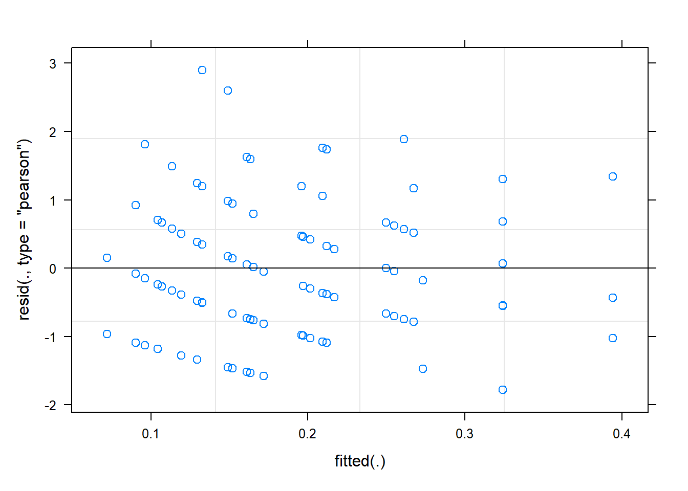
The discrete nature of the observations is visible, but otherwise most of the residuals seem within the limits we expect them to be [-2, 2]. They may have a wider spread in the low range of the fitted values than in the higher range, but that could be due to the fewer point we have on that end.
To interpret the coefficients we need to back-transform with the inverse logit. This works only on the absolute values. So before back-transforming, we need to either add coefficients to the intercept, or use predict The latter is preferable, as it is a more generic solution and has an other advantage we’ll see later.
To predict, we first have to define what we want to predict. In this case the absolute levels of the 6 treatments. Hence we start with creating a data frame that has these 6 levels. We conveniently derive this from the data set.
dftopredict <- ds.cd %>% select(treatment) %>% distinct()We use this as newdata in a predict function. The argument re.form = NA indicates that the prediction will ignore random effects (meaning that the prediction is also reliable outside the context of these wells and runs of this trial, see companion text on LMM).
preds.m1.glmer <- predict(m1.glmer,newdata=dftopredict,re.form=NA)
preds.m1.glmer
1 2 3 4 5 6
-2.016453 -1.703170 -1.582276 -1.611648 -1.033287 -1.338339 This we still have to back-transform via the inverse logit.
preds.m1.glmer %>% inv_logit() 1 2 3 4 5 6
0.1174863 0.1540518 0.1704734 0.1663599 0.2624474 0.2077833 More conveniently, we can also ask for the prediction on the scale of the data that we provided the model, eliminating the need to manually back-transform.
predict(m1.glmer,newdata=dftopredict,re.form=NA, type = "response") 1 2 3 4 5 6
0.1174863 0.1540518 0.1704734 0.1663599 0.2624474 0.2077833 The predictions are now on the scale of proportions, with 11.7% infected wells (12 * 0.117 = 1.41) for the reference and 26.2% for treatment T4 (12 * 0.262 = 3.15), what corresponds to the raw means in the graph.
To keep track of what is what:
preds.m1.glmer <- dftopredict %>% mutate(pred.glmer = predict(m1.glmer,newdata=dftopredict,re.form=NA, type = "response"))So far the easy part. Obtaining contrast and confidence intervals on predictions and contrasts will be more difficult. We will come back to this once we introduced the other approaches.
3.1.2 Binomial model with brm
The function brm of the package brms fits full bayesian models via hamiltonian monte carlo sampling. Again, the details are not important in this course, but remember only that the solution these models provide come in the form of a large sample of possible values for all model parameters simultaneously, more concretely a large matrix with as many columns as the model has parameters and as many rows as we ask the algorithm to provide for us. This sample represents the posterior distribution of the solution, without that we need to know a formal definition of this distribution (which is the case for the maximum likelihood based model of glmer).
It means also that we will need to do some post-processing to get concise and easy interpretable output. You will see that this ‘post-processing’ is needed for all three approaches when more advanced output is needed from this models. In the case of brm it is even needed for the basic output.
We start by loading packages (brms uses rstan in the back ground; tidybayes is handy in the postprocessing). Add also the rstan-options line (see rstan if you want to know why).
The function call of brm looks very much like the one of glmer. It differs in the way the Y-variable is provided. Not a matrix but a specific notation infected|trials(ntot) that indicates the number positive cases over the total number of trials (Note: difference with glmer that requires matrix of success vs non-sucesses). Furthermore, we indicate that we require 3000 posterior samples (iter = 3000) and that we do this 4 times (chains = 4). However, we discard of each chain the first 1000 as warm up, leaving a total of 8000. You can conveniently distribute this over several cores (We usually let one chain run on one core.)
library(brms)Loading required package: RcppWarning: package 'Rcpp' was built under R version 4.2.3Loading 'brms' package (version 2.19.2). Useful instructions
can be found by typing help('brms'). A more detailed introduction
to the package is available through vignette('brms_overview').
Attaching package: 'brms'The following object is masked from 'package:lme4':
ngrpsThe following object is masked from 'package:stats':
arlibrary(rstan)Warning: package 'rstan' was built under R version 4.2.3Loading required package: StanHeadersWarning: package 'StanHeaders' was built under R version 4.2.3
rstan version 2.26.22 (Stan version 2.26.1)For execution on a local, multicore CPU with excess RAM we recommend calling
options(mc.cores = parallel::detectCores()).
To avoid recompilation of unchanged Stan programs, we recommend calling
rstan_options(auto_write = TRUE)
For within-chain threading using `reduce_sum()` or `map_rect()` Stan functions,
change `threads_per_chain` option:
rstan_options(threads_per_chain = 1)Do not specify '-march=native' in 'LOCAL_CPPFLAGS' or a Makevars file
Attaching package: 'rstan'The following object is masked from 'package:tidyr':
extractlibrary(tidybayes)Warning: package 'tidybayes' was built under R version 4.2.3
Attaching package: 'tidybayes'The following objects are masked from 'package:brms':
dstudent_t, pstudent_t, qstudent_t, rstudent_trstan_options(auto_write=TRUE)
m1.brm <- brm(data=ds.cd, infected|trials(ntot) ~ treatment + (1|week),family = binomial(link="logit"),
chains = 4,cores = 4, iter=3000, warmup = 1000)Compiling Stan program...Start samplingWarning: There were 6 divergent transitions after warmup. See
https://mc-stan.org/misc/warnings.html#divergent-transitions-after-warmup
to find out why this is a problem and how to eliminate them.Warning: Examine the pairs() plot to diagnose sampling problemsLike for most of the model objects, summary() provides an overview.
summary(m1.brm)Warning: There were 6 divergent transitions after
warmup. Increasing adapt_delta above 0.8 may help. See
http://mc-stan.org/misc/warnings.html#divergent-transitions-after-warmup Family: binomial
Links: mu = logit
Formula: infected | trials(ntot) ~ treatment + (1 | week)
Data: ds.cd (Number of observations: 120)
Draws: 4 chains, each with iter = 3000; warmup = 1000; thin = 1;
total post-warmup draws = 8000
Group-Level Effects:
~week (Number of levels: 5)
Estimate Est.Error l-95% CI u-95% CI Rhat Bulk_ESS Tail_ESS
sd(Intercept) 0.72 0.35 0.29 1.64 1.00 1811 2655
Population-Level Effects:
Estimate Est.Error l-95% CI u-95% CI Rhat Bulk_ESS Tail_ESS
Intercept -2.01 0.39 -2.81 -1.20 1.00 1863 2325
treatmentT1 0.32 0.26 -0.18 0.85 1.00 3599 5025
treatmentT2 0.45 0.26 -0.04 0.95 1.00 3421 4905
treatmentT3 0.41 0.26 -0.10 0.92 1.00 3652 5406
treatmentT4 1.00 0.24 0.53 1.48 1.00 3214 4597
treatmentT5 0.69 0.25 0.20 1.18 1.00 3564 4473
Draws were sampled using sampling(NUTS). For each parameter, Bulk_ESS
and Tail_ESS are effective sample size measures, and Rhat is the potential
scale reduction factor on split chains (at convergence, Rhat = 1).The output is, not unexpectedly, similar as the one of glmer. Also here we find the group-level effects (or random effects in the world of glmer) and the coefficients of the fixed effects, equally on the scale of the model. There are no p-values but the credible intervals indicate that both T4 and T5 are significantly different from the reference.
The new additions here are the column Rhat which is a measure of the convergence and should be one (or very close to it) and the effective sample size ESS. These numbers have to be compared to the number of requested samples.
The brms objects have also a predict method. In this case, the actual counts are predicted. Hence the total wells needs to be included in newdata. We set this to a high number we don’t get bothered by rounding issues.
Just like for glmer we indicate that we do not condition on the random effects.
This predict will by default return value on the backtransformed scale. Nothing to worry about.
preds.m1.brm <- bind_cols(dftopredict, predict(m1.brm,newdata=data.frame(dftopredict,ntot=1000),re_formula = NA)/1000)
preds.m1.brm %>% mutate(across(where(is.numeric),~round(.,3)))
treatment Estimate Est.Error Q2.5 Q97.5
1 reference 0.124 0.045 0.055 0.235
2 T1 0.163 0.054 0.074 0.291
3 T2 0.180 0.059 0.083 0.317
4 T3 0.175 0.058 0.080 0.311
5 T4 0.273 0.075 0.141 0.441
6 T5 0.218 0.066 0.105 0.372Let’s demonstrate the last package.
3.1.3 Binomial model with inla
The syntax of inla is rather different. The random grouping effect has to be provided via an idd model in the f() function. The total number of cells has to be provided via as separate argument Ntrials.
library(INLA)Loading required package: foreach
Attaching package: 'foreach'The following objects are masked from 'package:purrr':
accumulate, whenLoading required package: parallelLoading required package: spWarning: package 'sp' was built under R version 4.2.3This is INLA_22.05.07 built 2022-05-07 09:52:03 UTC.
- See www.r-inla.org/contact-us for how to get help.m1.inla <- inla(data=ds.cd, infected ~ treatment + f(week, model = "iid"), Ntrials= ntot,
family="binomial",
control.family = list(control.link=list(model="logit")),
control.compute=list(config=TRUE)
)
m1.inla.abs <- inla(data=ds.cd, infected ~ 0 + treatment + f(week, model = "iid"), Ntrials= ntot,
family="binomial",
control.family = list(control.link=list(model="logit")),
control.compute=list(config=TRUE)
)The summary() leads to similar output as before. Be aware that variance are presented as precisions: the inverse of variances. E.g the estimation of the week variability is 1/8.116 or a sd of 0.35.
summary(m1.inla)
Call:
   c("inla.core(formula = formula, family = family, contrasts = contrasts,
   ", " data = data, quantiles = quantiles, E = E, offset = offset, ", "
   scale = scale, weights = weights, Ntrials = Ntrials, strata = strata,
   ", " lp.scale = lp.scale, link.covariates = link.covariates, verbose =
   verbose, ", " lincomb = lincomb, selection = selection, control.compute
   = control.compute, ", " control.predictor = control.predictor,
   control.family = control.family, ", " control.inla = control.inla,
   control.fixed = control.fixed, ", " control.mode = control.mode,
   control.expert = control.expert, ", " control.hazard = control.hazard,
   control.lincomb = control.lincomb, ", " control.update =
   control.update, control.lp.scale = control.lp.scale, ", "
   control.pardiso = control.pardiso, only.hyperparam = only.hyperparam,
   ", " inla.call = inla.call, inla.arg = inla.arg, num.threads =
   num.threads, ", " blas.num.threads = blas.num.threads, keep = keep,
   working.directory = working.directory, ", " silent = silent, inla.mode
   = inla.mode, safe = FALSE, debug = debug, ", " .parent.frame =
   .parent.frame)")
Time used:
    Pre = 1.04, Running = 0.343, Post = 0.126, Total = 1.51
Fixed effects:
              mean    sd 0.025quant 0.5quant 0.975quant mode kld
(Intercept) -2.017 0.286     -2.597   -2.011     -1.466   NA   0
treatmentT1  0.313 0.265     -0.202    0.312      0.836   NA   0
treatmentT2  0.434 0.260     -0.072    0.432      0.949   NA   0
treatmentT3  0.405 0.261     -0.104    0.403      0.922   NA   0
treatmentT4  0.983 0.246      0.508    0.980      1.474   NA   0
treatmentT5  0.678 0.253      0.188    0.675      1.181   NA   0

Random effects:
  Name    Model
    week IID model

Model hyperparameters:
                   mean   sd 0.025quant 0.5quant 0.975quant mode
Precision for week 8.12 6.50       1.32     6.45      24.39   NA

Marginal log-Likelihood:  -232.39
 is computed
Posterior summaries for the linear predictor and the fitted values are computed
(Posterior marginals needs also 'control.compute=list(return.marginals.predictor=TRUE)')
preds.m1.inla <- m1.inla.abs$summary.fixed %>%
as_tibble(rownames="treatment") %>% mutate(treatment=gsub("treatment","",treatment)) %>%
mutate(pred.inla=inv_logit(mean)) %>%
select(treatment,pred.inla)
preds.m1.inla %>% mutate(across(where(is.numeric),~round(.,3)))# A tibble: 6 × 2
treatment pred.inla
<chr> <dbl>
1 reference 0.118
2 T1 0.154
3 T2 0.171
4 T3 0.167
5 T4 0.263
6 T5 0.2083.1.4 Comparison of the predictions
rmean <- ds.cd %>% group_by(treatment) %>% summarise(rawmean=mean(infected/ntot))
comparison  <- inner_join(rmean,preds.m1.glmer,by="treatment") %>%
               inner_join(preds.m1.brm %>% select("treatment","Estimate") %>% rename(pred.brms="Estimate"),by="treatment") %>% inner_join(preds.m1.inla,by="treatment")

comparison %>% mutate(across(where(is.numeric),~round(.,3)))
# A tibble: 6 × 5
treatment rawmean pred.glmer pred.brms pred.inla
<chr> <dbl> <dbl> <dbl> <dbl>
1 reference 0.125 0.117 0.124 0.118
2 T1 0.162 0.154 0.163 0.154
3 T2 0.179 0.17 0.18 0.171
4 T3 0.175 0.166 0.175 0.167
5 T4 0.271 0.262 0.273 0.263
6 T5 0.217 0.208 0.218 0.208From this simple comparison (based on a single data set…) we see that the approximate methods (glmer and inla) produce identical estimates that not entirely agree with the brms-estimates, but that brms stays closest to the raw means.