5 Other families
5.1 Data set : Cell discolouration
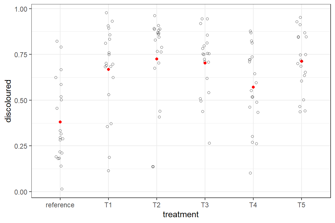
Suppose that another methodology to evaluate the virulence would be to grow the cells in a larger plate and score cell death via imaging and proportion of the plate surface covered with discoloured cells. The data are shown in the graph below as the black dots. The red dots are simple averages.
to download the data: here
The data are proportions. Proportions (constrained on both sides of its range) can be treated via a beta error distribution.
There is a caveat for using this distribution: although the data are constrained by two limits (in this case 0 and 1) the data should not contain those limits. In the case of this computer vision that may not be an issue, but visual assessments can have total absence or complete discolouration. If so a transformation needs to be done that squeezes all data inward. See how you can do this in the chunk below.It is demonstrated on a data set of 100 proportions with 4 of them either 0 or 1. We show only the first 10 data points. The values around 0.5 do not change but the more extreme are shrunken toward 0.5, with the largest shift for the zeros and ones.
transformforbeta <- function (y) {

  if(all(y > 0 & y < 1 )) {
    return(y)
  } else {
  n <- length(y)
    return((y*(n-1) + 0.5)/n)
  }
}

x <- c(0,0,1,1,runif(96))
round(x[1:10],3)
[1] 0.000 0.000 1.000 1.000 0.963 0.091 0.633 0.799 0.996 0.648round(transformforbeta(x)[1:10],3) [1] 0.005 0.005 0.995 0.995 0.959 0.095 0.632 0.796 0.991 0.646Because the virulence data set does not contains zero or ones, the line of code below will have no impact.
ds.ip <- ds.ip %>% mutate(discoloured=transformforbeta(discoloured))The beta distribution has two parameters, but the parametrisation of beta distributions come in two forms. The two parameter are either two shape parameters (as used for instance by the rbeta() or dbeta() function in the R stats base package) or a mean (mu) and a second parameter called phi that lets the spread to vary. This phi has the behavior of a precision, i.e. the inverse of a variance. So the larger, the narrower the distribution. See the appendix for some examples. This mu-phi parametrisation is used by brms and inla, and hence we will use it here.
This parametrisation also brings about the similarity with fitting models based on a normal error distribution, which has also a mean and a variance. When fitting an anova we assume there is one common variance, and focus on the means. Only when the assumption of homoscedasticity (equal variance) cannot be supported, heteroscedastic models where both the means and variance can vary, albeit not necessarily along the same factors. For instance, in data sets with increasing variance for higher values, the mean can be estimate for the different treatments, whereas the variance is modelled according to the fitted values.
A similar reasoning is followed here for the beta regression. The standard solution could be separate mu’s and one common phi, but in some cases we can opt for varying phi albeit with a different model and in this situation even a different link family.
5.1.1 Beta regression with brm
Below the code for three beta regressions with brms. Model m6.brm is the base model for which phi is considered as common over all treatments (the default). Model m7.brm and model m8.brm are two alternative models in which phi is modelled either by treatment or by the random effect of week.
m6.brm <- brm(data=ds.ip, discoloured ~ treatment + (1|week),
          family = Beta(link="logit",link_phi = "log"),
          chains = 4,cores = 4, iter=3000, warmup = 1000)
Compiling Stan program...Start samplingWarning: There were 6 divergent transitions after warmup. See
https://mc-stan.org/misc/warnings.html#divergent-transitions-after-warmup
to find out why this is a problem and how to eliminate them.Warning: Examine the pairs() plot to diagnose sampling problemssummary(m6.brm)Warning: There were 6 divergent transitions after
warmup. Increasing adapt_delta above 0.8 may help. See
http://mc-stan.org/misc/warnings.html#divergent-transitions-after-warmup Family: beta
Links: mu = logit; phi = identity
Formula: discoloured ~ treatment + (1 | week)
Data: ds.ip (Number of observations: 120)
Draws: 4 chains, each with iter = 3000; warmup = 1000; thin = 1;
total post-warmup draws = 8000
Group-Level Effects:
~week (Number of levels: 5)
Estimate Est.Error l-95% CI u-95% CI Rhat Bulk_ESS Tail_ESS
sd(Intercept) 0.15 0.14 0.01 0.52 1.00 2566 3511
Population-Level Effects:
Estimate Est.Error l-95% CI u-95% CI Rhat Bulk_ESS Tail_ESS
Intercept -0.52 0.22 -0.95 -0.11 1.00 2892 4017
treatmentT1 1.21 0.29 0.64 1.77 1.00 4315 4530
treatmentT2 1.42 0.28 0.87 2.00 1.00 3710 5287
treatmentT3 1.32 0.28 0.77 1.88 1.00 3769 5241
treatmentT4 0.78 0.28 0.23 1.35 1.00 3684 5012
treatmentT5 1.35 0.29 0.77 1.91 1.00 4269 5308
Family Specific Parameters:
Estimate Est.Error l-95% CI u-95% CI Rhat Bulk_ESS Tail_ESS
phi 4.21 0.50 3.29 5.24 1.00 5668 5141
Draws were sampled using sampling(NUTS). For each parameter, Bulk_ESS
and Tail_ESS are effective sample size measures, and Rhat is the potential
scale reduction factor on split chains (at convergence, Rhat = 1).The output is very similar as what we had before. There is now extra output to show the estimate of phi (in this model a single unique estimate). In order to have interpretable numbers for the fixed effects from this fit we still need to backtransform (the inverse logit), exactly the same way as was shown for the binomial model earlier.
The phi parameter is already on the scale of the measurement. Hence no need for back transformation.
The output of the two alternative models looks a bit different and depends how the phi was modelled.
m7.brm <- brm(data=ds.ip,
             bf(discoloured ~ treatment + (1|week),
              phi ~ treatment),
          family = Beta(link="logit",link_phi = "log"),
          chains = 4,cores = 4, iter=3000, warmup = 1000)
Compiling Stan program...Start samplingWarning: There were 18 divergent transitions after warmup. See
https://mc-stan.org/misc/warnings.html#divergent-transitions-after-warmup
to find out why this is a problem and how to eliminate them.Warning: Examine the pairs() plot to diagnose sampling problemssummary(m7.brm)Warning: There were 18 divergent transitions after
warmup. Increasing adapt_delta above 0.8 may help. See
http://mc-stan.org/misc/warnings.html#divergent-transitions-after-warmup Family: beta
Links: mu = logit; phi = log
Formula: discoloured ~ treatment + (1 | week)
phi ~ treatment
Data: ds.ip (Number of observations: 120)
Draws: 4 chains, each with iter = 3000; warmup = 1000; thin = 1;
total post-warmup draws = 8000
Group-Level Effects:
~week (Number of levels: 5)
Estimate Est.Error l-95% CI u-95% CI Rhat Bulk_ESS Tail_ESS
sd(Intercept) 0.20 0.19 0.01 0.70 1.00 1679 848
Population-Level Effects:
Estimate Est.Error l-95% CI u-95% CI Rhat Bulk_ESS Tail_ESS
Intercept -0.49 0.24 -0.96 -0.02 1.00 2008 1783
phi_Intercept 1.23 0.29 0.63 1.79 1.00 2888 3575
treatmentT1 1.12 0.32 0.50 1.73 1.00 3702 5253
treatmentT2 1.31 0.32 0.68 1.93 1.00 3345 4845
treatmentT3 1.33 0.29 0.75 1.89 1.00 2900 4425
treatmentT4 0.74 0.30 0.15 1.33 1.00 3413 4960
treatmentT5 1.40 0.28 0.84 1.94 1.00 3036 4707
phi_treatmentT1 -0.08 0.41 -0.89 0.74 1.00 3741 4214
phi_treatmentT2 -0.07 0.42 -0.89 0.76 1.00 3561 4500
phi_treatmentT3 0.55 0.43 -0.30 1.41 1.00 3570 4215
phi_treatmentT4 0.20 0.41 -0.61 1.01 1.00 3867 4931
phi_treatmentT5 0.72 0.44 -0.13 1.57 1.00 3560 5010
Draws were sampled using sampling(NUTS). For each parameter, Bulk_ESS
and Tail_ESS are effective sample size measures, and Rhat is the potential
scale reduction factor on split chains (at convergence, Rhat = 1).m8.brm <- brm(data=ds.ip,
bf(discoloured ~ treatment + (1|week),
phi ~ (1|week)),
family = Beta(link="logit",link_phi = "log"),
chains = 4,cores = 4, iter=3000, warmup = 1000)Compiling Stan program...Start samplingWarning: There were 12 divergent transitions after warmup. See
https://mc-stan.org/misc/warnings.html#divergent-transitions-after-warmup
to find out why this is a problem and how to eliminate them.Warning: Examine the pairs() plot to diagnose sampling problemssummary(m8.brm)Warning: There were 12 divergent transitions after
warmup. Increasing adapt_delta above 0.8 may help. See
http://mc-stan.org/misc/warnings.html#divergent-transitions-after-warmup Family: beta
Links: mu = logit; phi = log
Formula: discoloured ~ treatment + (1 | week)
phi ~ (1 | week)
Data: ds.ip (Number of observations: 120)
Draws: 4 chains, each with iter = 3000; warmup = 1000; thin = 1;
total post-warmup draws = 8000
Group-Level Effects:
~week (Number of levels: 5)
Estimate Est.Error l-95% CI u-95% CI Rhat Bulk_ESS Tail_ESS
sd(Intercept) 0.18 0.18 0.01 0.63 1.00 1431 2476
sd(phi_Intercept) 0.34 0.30 0.01 1.15 1.00 1449 807
Population-Level Effects:
Estimate Est.Error l-95% CI u-95% CI Rhat Bulk_ESS Tail_ESS
Intercept -0.57 0.23 -1.03 -0.13 1.00 2228 2821
phi_Intercept 1.46 0.23 1.03 1.98 1.01 1372 633
treatmentT1 1.30 0.30 0.72 1.92 1.00 3023 2516
treatmentT2 1.51 0.30 0.92 2.10 1.00 2763 3024
treatmentT3 1.40 0.30 0.82 1.99 1.00 3414 3920
treatmentT4 0.82 0.29 0.27 1.40 1.00 3206 2703
treatmentT5 1.43 0.30 0.85 2.01 1.00 2928 2893
Draws were sampled using sampling(NUTS). For each parameter, Bulk_ESS
and Tail_ESS are effective sample size measures, and Rhat is the potential
scale reduction factor on split chains (at convergence, Rhat = 1).When comparing the 3 beta models via the leave-one-out crossvalidaton, it turns out that there is no additional value to model phi in a more complex manner.
loo(m6.brm,m7.brm,m8.brm)Warning: Found 1 observations with a pareto_k > 0.7 in model 'm8.brm'. It is
recommended to set 'moment_match = TRUE' in order to perform moment matching for
problematic observations.Output of model 'm6.brm':
Computed from 8000 by 120 log-likelihood matrix
Estimate SE
elpd_loo 23.5 7.2
p_loo 8.4 1.4
looic -47.1 14.4
------
Monte Carlo SE of elpd_loo is 0.0.
All Pareto k estimates are good (k < 0.5).
See help('pareto-k-diagnostic') for details.
Output of model 'm7.brm':
Computed from 8000 by 120 log-likelihood matrix
Estimate SE
elpd_loo 20.6 7.0
p_loo 14.2 2.2
looic -41.2 14.1
------
Monte Carlo SE of elpd_loo is 0.1.
Pareto k diagnostic values:
Count Pct. Min. n_eff
(-Inf, 0.5] (good) 114 95.0% 1327
(0.5, 0.7] (ok) 6 5.0% 437
(0.7, 1] (bad) 0 0.0% <NA>
(1, Inf) (very bad) 0 0.0% <NA>
All Pareto k estimates are ok (k < 0.7).
See help('pareto-k-diagnostic') for details.
Output of model 'm8.brm':
Computed from 8000 by 120 log-likelihood matrix
Estimate SE
elpd_loo 22.5 7.7
p_loo 11.5 2.2
looic -44.9 15.5
------
Monte Carlo SE of elpd_loo is NA.
Pareto k diagnostic values:
Count Pct. Min. n_eff
(-Inf, 0.5] (good) 118 98.3% 623
(0.5, 0.7] (ok) 1 0.8% 2841
(0.7, 1] (bad) 1 0.8% 124
(1, Inf) (very bad) 0 0.0% <NA>
See help('pareto-k-diagnostic') for details.
Model comparisons:
elpd_diff se_diff
m6.brm 0.0 0.0
m8.brm -1.1 1.4
m7.brm -2.9 2.3 5.1.2 Beta regression with inla
For the record, model m6 in an inla-version
m6.inla <- inla(data=ds.ip, discoloured ~ treatment + f(week, model = "iid"),
           family="beta",
           control.family = list(control.link=list(model="logit")),
           control.compute=list(config=TRUE)
            )

summary(m6.inla)
Call:
   c("inla.core(formula = formula, family = family, contrasts = contrasts,
   ", " data = data, quantiles = quantiles, E = E, offset = offset, ", "
   scale = scale, weights = weights, Ntrials = Ntrials, strata = strata,
   ", " lp.scale = lp.scale, link.covariates = link.covariates, verbose =
   verbose, ", " lincomb = lincomb, selection = selection, control.compute
   = control.compute, ", " control.predictor = control.predictor,
   control.family = control.family, ", " control.inla = control.inla,
   control.fixed = control.fixed, ", " control.mode = control.mode,
   control.expert = control.expert, ", " control.hazard = control.hazard,
   control.lincomb = control.lincomb, ", " control.update =
   control.update, control.lp.scale = control.lp.scale, ", "
   control.pardiso = control.pardiso, only.hyperparam = only.hyperparam,
   ", " inla.call = inla.call, inla.arg = inla.arg, num.threads =
   num.threads, ", " blas.num.threads = blas.num.threads, keep = keep,
   working.directory = working.directory, ", " silent = silent, inla.mode
   = inla.mode, safe = FALSE, debug = debug, ", " .parent.frame =
   .parent.frame)")
Time used:
    Pre = 1.01, Running = 0.319, Post = 0.216, Total = 1.55
Fixed effects:
              mean    sd 0.025quant 0.5quant 0.975quant mode kld
(Intercept) -0.504 0.197     -0.897   -0.502     -0.124   NA   0
treatmentT1  1.195 0.281      0.648    1.194      1.753   NA   0
treatmentT2  1.402 0.285      0.850    1.400      1.967   NA   0
treatmentT3  1.296 0.283      0.746    1.294      1.857   NA   0
treatmentT4  0.763 0.277      0.223    0.762      1.310   NA   0
treatmentT5  1.331 0.283      0.780    1.329      1.893   NA   0

Random effects:
  Name    Model
    week IID model

Model hyperparameters:
                                                  mean       sd 0.025quant
precision parameter for the beta observations     4.24 5.05e-01       3.32
Precision for week                            16763.29 1.60e+04    1087.09
                                              0.5quant 0.975quant mode
precision parameter for the beta observations     4.21       5.30   NA
Precision for week                            11879.99   59276.52   NA

Marginal log-Likelihood:  3.16
 is computed
Posterior summaries for the linear predictor and the fitted values are computed
(Posterior marginals needs also 'control.compute=list(return.marginals.predictor=TRUE)')
5.1.3 Beta regression in lme4
Beta error distributions are not implemented in lme4. The alternative R packages glmmTMB does handle more diverse error distributions than lme4. The beta distribution is one of them. See the documentation for glmmTMB.
5.2 Data set: seedling height
In a sowing experiment various seed treatments are tested to see whether they can enhance earlier development of the seedling. Seeds are individually sown in soil plugs. After 3 weeks the height of the seedlings is measured and majority ranges between 8 and 16 cm at that time. The height will be used to compare the treatments on their plant stimulating effect.
However, not all seeds germinated or the sprout never or hardly appeared at the surface. About 5% will never become a normal healthy plant. Some of this could be genetic defects, but it may have been caused by the seed treatment as well.
Ignore these seedlings could create a bias. Including all the zeros or very small numbers will render the error distribution not-normal.
The experiment tested 4 different seed coats (T1 to T4), each with 120 seeds, sown in 6 complete blocks.
Below histograms of the seedling height in cm after 3 weeks by seed coat. Plant height smaller than 3 cm were set to 0, as they will die off anyhow. There seem to be a block effect as well on the number of not properly established seedlings (height = 0).
ds.sd <- readRDS("_book/data/Seedlings.obj")
ds.sd %>% ggplot(aes(x=height)) +
  geom_histogram(binwidth=0.5) +
  facet_wrap(~seedcoat)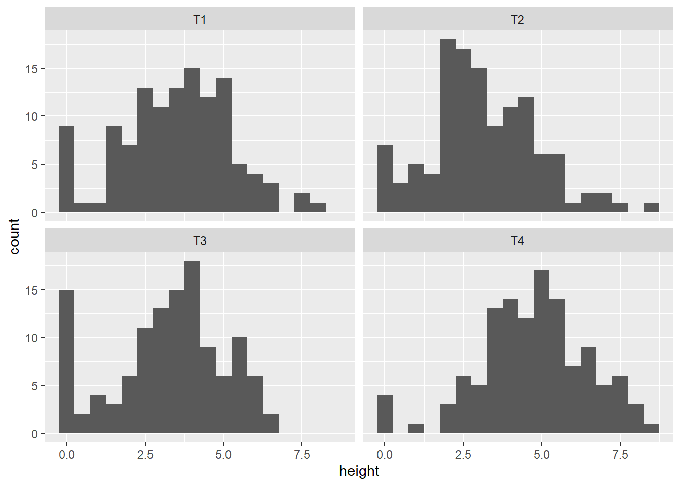
ds.sd %>% filter(height == 0) %>% group_by(Block) %>% count()# A tibble: 6 × 2
# Groups: Block [6]
Block n
<fct> <int>
1 B1 8
2 B2 7
3 B3 3
4 B4 4
5 B5 5
6 B6 7Below we model this data as a hurdle model to take care of the zeros and a lognormal distribution for the continous non-zero part of the heights.
m8.brm <- brm(data=ds.sd,
               bf(height ~ seedcoat + (1|Block),
                  hu ~ seedcoat + (1|Block)
               ),
               family = hurdle_lognormal(),
               iter = 2500,warmup = 500,
               control = list(adapt_delta = 0.95,max_treedepth = 10),
               chains = 4,cores = 4)
Compiling Stan program...Start samplingWarning: There were 1 divergent transitions after warmup. See
https://mc-stan.org/misc/warnings.html#divergent-transitions-after-warmup
to find out why this is a problem and how to eliminate them.Warning: Examine the pairs() plot to diagnose sampling problemssummary(m8.brm)Warning: There were 1 divergent transitions after
warmup. Increasing adapt_delta above 0.95 may help. See
http://mc-stan.org/misc/warnings.html#divergent-transitions-after-warmup Family: hurdle_lognormal
Links: mu = identity; sigma = identity; hu = logit
Formula: height ~ seedcoat + (1 | Block)
hu ~ seedcoat + (1 | Block)
Data: ds.sd (Number of observations: 480)
Draws: 4 chains, each with iter = 2500; warmup = 500; thin = 1;
total post-warmup draws = 8000
Group-Level Effects:
~Block (Number of levels: 6)
Estimate Est.Error l-95% CI u-95% CI Rhat Bulk_ESS Tail_ESS
sd(Intercept) 0.06 0.05 0.00 0.18 1.00 2424 3161
sd(hu_Intercept) 0.32 0.29 0.01 1.06 1.00 3041 3262
Population-Level Effects:
Estimate Est.Error l-95% CI u-95% CI Rhat Bulk_ESS Tail_ESS
Intercept 1.23 0.06 1.12 1.35 1.00 5275 4661
hu_Intercept -2.54 0.39 -3.32 -1.82 1.00 6544 5931
seedcoatT2 -0.16 0.07 -0.30 -0.02 1.00 7102 6171
seedcoatT3 -0.07 0.07 -0.21 0.07 1.00 6960 5698
seedcoatT4 0.30 0.07 0.16 0.43 1.00 7238 6329
hu_seedcoatT2 -0.29 0.53 -1.36 0.74 1.00 7334 5197
hu_seedcoatT3 0.49 0.45 -0.39 1.39 1.00 7403 6126
hu_seedcoatT4 -0.90 0.63 -2.23 0.29 1.00 7599 5558
Family Specific Parameters:
Estimate Est.Error l-95% CI u-95% CI Rhat Bulk_ESS Tail_ESS
sigma 0.53 0.02 0.50 0.57 1.00 10918 6365
Draws were sampled using sampling(NUTS). For each parameter, Bulk_ESS
and Tail_ESS are effective sample size measures, and Rhat is the potential
scale reduction factor on split chains (at convergence, Rhat = 1).nd <- ds.sd %>% select(seedcoat) %>% distinct()
fit.m8.brm <- bind_cols(nd,fitted(m8.brm,newdata=nd,summary=TRUE,scale="response",re_formula = NA))
fit.m8.brm seedcoat Estimate Est.Error Q2.5 Q97.5
1 T1 3.654191 0.2415263 3.195151 4.140889
2 T2 3.170830 0.2020734 2.787290 3.586448
3 T3 3.244804 0.2285700 2.802152 3.710929
4 T4 5.155251 0.3121723 4.567153 5.791892To check what the difference is with fitting a general linear model with
- all data ignoring the fact that there are many zeros
- data filtered heights > 0
m8.lmer <- lmer(data=ds.sd,
                height ~ seedcoat + (1|Block)
               )
boundary (singular) fit: see help('isSingular')fits.m8 <- bind_cols(nd,pred.hu = fit.m8.brm$Estimate, pred.all = predict(m8.lmer,newdata=nd,re.form = NA))m8bis.lmer <- lmer(data=ds.sd %>% filter(height >0),
height ~ seedcoat + (1|Block)
)
fits.m8 <- bind_cols(fits.m8,pred.wozero = predict(m8bis.lmer,newdata=nd,re.form = NA))
fits.m8 seedcoat pred.hu pred.all pred.wozero
1 T1 3.654191 3.492267 3.775557
2 T2 3.170830 3.152294 3.348147
3 T3 3.244804 3.221363 3.646893
4 T4 5.155251 4.736259 4.900647