2  The family and its role in GLMM

The family argument is usually provided by a function. For instance for the classic linear model the default family is provided as:

family = gaussian(link = "identity")

hence the function gaussian with the argument link set to “identity”.

Other families are available e.g. an alternative could be

family = poisson(link = "log")

To understand why a distribution and a link is needed we have to go back to how linear models work.

For classic linear models, a given observation $y_i$ can be represented by its modelled mean ${\mu }_i$ plus a residual drawn from a normal distribution $$y_i\sim {\mu }_i+normal(0,\sigma )$$ or $$y_i\sim normal({\mu }_i,\sigma )$$ The ${\mu }_i$ is itself modelled by general constant $\alpha$, and series of coefficients of which some may be multipliers ($\beta$) for an attribute $x$ of the sample where $y_i$ is observed on. $$\mu \mathrm{\_}i=\alpha +{\beta }_i{x}_i$$ For instance, a volume of a 15-year old tree ($y_i$ = 3.62) is represented by $3.62={\mu }_i+e_i=3.34+0.28$

• where ${\mu }_i=0.1+0.21\ast 15=3.34$ for a starting volume of 0.1 plus an increase of 0.21 for each year.
• and $e_i=0.28$ forms together with all other $e$ a normal distribution with mean 0 and standard deviation $\sigma$.

For generalized linear models, this base structure remains but is generalized to:

$$y_i\sim thefamily({\mu }_i,distribution\mathrm{\_}parameters)$$

So whatever distribution for the likelihood of the residuals with its particular parameters, the modelling is done of the link-transformed ${\mu }_i$ but still according to a linear combination of coefficients and the attributes of the observed samples.

$$link({\mu }_i)=\alpha +{\beta }_i{x}_i$$

In the classic case the link function was just the identity function, so no transformation at all. In other words in the classic model the actual $\mu$’s are modelled.

For example, rabbit litter counts, where the mothers are given one of two diets could be modelled via a poisson regression with $log$ as link function. This would give:

$$littersiz{e}_i\sim poisson({\mu }_i)$$ (the poisson distribution has only the mean as parameter, so no other to be defined here) and

$$log({\mu }_i)=\alpha +\beta {\ast }^{\prime }isonalternativedie{t}^{\prime })$$ with ‘is on alternative diet’ is either 0 or 1. Hence the logs of mean litter sizes are modelled and $\beta$ would be the average additional log(kit) that the alternative diet adds to the average log(kit) of litters on the reference diet. Or with a bit of maths background (remember that $log(a)-log(b)=log(a/b)$) you get that $\beta$ is the multiplier to go from the actual number of litter size on the reference diet to the actual sizes of litters on the alternative diet. The model provides a proportional increase rather than an added effect.

This log link function is handy because it avoids that the model goes in the negative domain (there are no negative litter sizes) but at the same time it complicates the interpretation. That complication can be easy to handle (back transformation by exponentiation in this case) but in more elaborate models interpretation of the model outcome will become an issue.

Another common link function is the logit function. It is an interesting transformation because it keeps prediction within a range between 0 and 1. The logit is defined as:

$$logit(p)=ln(\frac{p}{1-p})$$

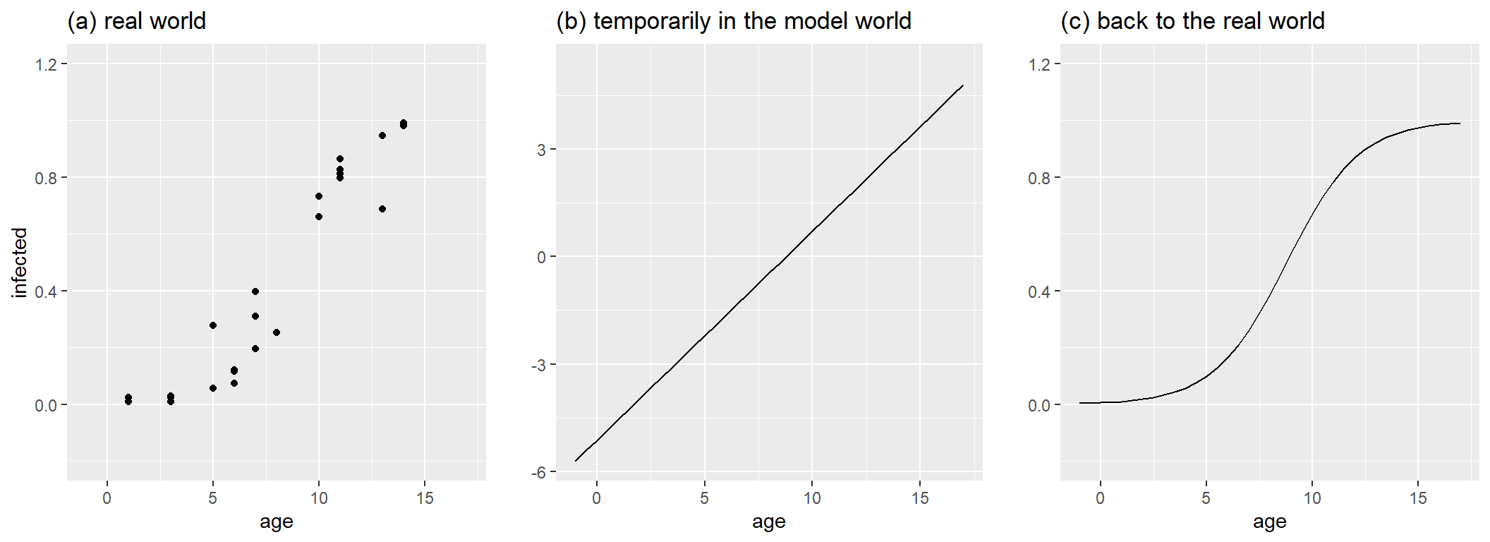
To show what its role is, suppose that the trees we mentioned earlier can get infected by a fungus. The older the tree gets, the higher the chances on infection. We collect 200 leaves of each tree and count the number infected ones and calculate the proportion of infected leaves.

In the figure below on the left, the original observations are plotted. They are confined between 0 and 1: no less then 0 leaves can be infected and if all leaves are infected, the proportion becomes 1 and not higher. With a bit of good will, we could just fit a linear regression through the dots. However, that would mean that a tree of 20 years old has a probability of >1 to be infected. For a 2-year old tree, that probability would be negative. With a more appropriate generalized linear model we avoid these problems. For the modelling, a shift to the logit scale allows to model the impact of age with a simple linear model (middle graph). Yet, to interpret the outcome on an understandable scale and to make sure that that the proportion is not increasing above 1 when trees would become 20 or 25 years old, the inverse of the logit is applied, leading to the s-curve on the right.

(a) $\to$ logit $\to$ linear model $\to$ (b) $\to$ inverse logit $\to$ (c)

The inverse logit you could have derived yourself, but for convenience:

$$inverse\mathrm{\_}logit(\mu )=\frac{exp(\mu )}{1+exp(\mu )}$$

2.1 Why make it so complicated?

This is all fine, but what is the difference with applying the transformation directly on the data and proceed with a general linear (mixed) model? Well, in that approach we would hope that the variables become normally distributed. That could be approximately a valid assumption in some case, but not in many others, e.g a discrete distribution will not become continuous by transforming it. In GLMM it are the means or coefficients that are transformed by the link function, not the original observations. That makes a difference. The mean of logs of something is not equal to the log of the mean.

log(mean(c(1,4,6)))

[1] 1.299283

mean(c(log(1),log(4),log(6)))

[1] 1.059351

And that shows in a comparison between two very simple models on these data.

dd <- c(1,4,6)
mean(dd)

[1] 3.666667

The direct mean gives 3.67

The respective alternative approaches:

# lm on log transformed data
mod.lm <- lm(log(dd)~1)
coefficients(mod.lm)

(Intercept) 
   1.059351 

#backtransformed:
exp(coefficients(mod.lm))

(Intercept) 
   2.884499 

# glm with log link
mod.glm <- glm(dd~1, family = poisson(link="log"))
coefficients(mod.glm)

(Intercept) 
   1.299283 

# what gives backtransformed:
exp(coefficients(mod.glm))

(Intercept) 
   3.666667 

Hence, the glm conserved the mean on the raw values.

Sometimes it does make sense to transform the data, when the transformed scale has a clear meaning and directly interpretable. For instance, the square root of an area or the cube-root of a volumes gives a length. The -log of the molarity of H+ ions is called a pH.

If you haven’t grasped everything in the previous paragraph, no worries. The important part to remember that we will have to provide a family with its likelihood and a link function, and that the fact that we work on the transformed scale of that link function will require us to back-transform which can be cumbersome. A problem we will solve later.

2.2 The choice of the family and link function

It should be clear by now that the family and link function play a pivotal role, yet there is quite some diversity among these families. How do you choose them?

There may be theoretical reason to choose one distribution over another, or have a clear preference for some link function (times-to-event are often modelled with a gamma distribution because the theoretical build-up of gamma distributions).

Yet, most practical is to base the decision on the type of observations and exploring the obtained data. There exist methods to check whether the choice you made, is sensible, but usually one is selected from the basic set given below. Moreover, some of the more general libraries in R will only provide (some of) these distributions. For more exotic distributions specialized packages are required. For instance, circular data (wind direction, events on the circadian clock) with the start and end of the scale coinciding, require special attention.

So, pragmatically: ask yourself whether your data are continuous or not, whether they are constrained on one or both ends of the scale, whether they are skewed or not, and whether they contain more zero’s (or ones) than you would expect from a continuous distribution. If your data are not continuous, your choice will depend on the number of classes (2 classes, more than 2 classes and lots of classes) and whether they are ordered according to some scale. Than pick one out of the options in the following list:

1. Continuous data or data that behave as continuous data

When the obtained data are continuous measurements or when they are counts and all are well above 20, check if the data are skewed or come close to hard boundaries like 0 or 1 or 100. If that is not the case, the gaussian family will often be appropriate (i.e. a general linear model). For instance, if you have proportions but the obtained data seldom leave the range 0.3 - 0.7, you could try the simpler general linear model. When the data contains many large outliers an alternative is a student error distribution. For both gaussia and tudent the identity link is used (i.e. no transformation).

Often data in life sciences are positive or zero and right-skewed (majority of observations is below the mean and have a few very large values). When there is no hard boundary at the high end, a gamma error distribution with a log link is what you need. An alternative here is an inverse gaussian, with the link function $1/{\mu }^2$ or a lognormal with log link.

If the observations have hard boundary at zero and another hard boundary at their maximum (e.g. proportions), and you often get close to (one of) those boundaries, use a beta error distribution. (Remark: The beta family uses two link functions, logit and log.)

Remark: Don’t mix up a proportion that is directly obtained as a proportion (the part of a leaf covered by mould, the part of an experimental plot that is affected by a beetle, the part of a skin that is discoloured) with ratio’s that are obtained by dividing two numbers. Depending on the distribution of the numerator and denominator, whether they are counts or continuous, and whether the ratio can become larger than 1, the analysis will be very different; and many cases fall outside the scope of this text.

The distributions mentioned above have been illustrated in the appendix to this document.

2. Count data with presence of low integers

With count data we mean counts for which there is in principal no physical maximum. Such count data are often treated with a poisson error distribution, but a negative binomial distribution is usually the better choice as it offers more flexibility. The common link function in these cases is the log.

Counts of individual where you have a maximum (the number of broken eggs in a 6-egg tray, or counts of infected larvae where you can also count the non-infected larvae) belong to the next section.

3. Data in categories

Very often there are only two categories: yes/no, dead/alive, infected/not-infected. You have than counts of yes’s an counts of no’s. The data can be modelled via logistic regression, which is a generalized linear model with a binomial error distribution and the logit link function.

If you have more than two categories and those categories are in no particular order (blue, green, red or parties voted fro) multinomial or categorical families can be explored.

When those categories are ordered (healthy, slightly infected, heavily infected, almost dead) check out the cumulative family.

4. Data with lots of zeros

The presence of lots of zeros in the data causes trouble with fitting. An example is the amount of rain per day: on many days there is no rain at all, while on rainy days some quantity (often a little drizzle, once and a while a heavy thunderstorms) is recorded. Shoot length of infected seedlings in situations where a portion of the seeds does not germinate is another such case.

The zero’s can be structural (0 because the seed did not germinate at all) or because of the sampling and distribution (the seedling is so tiny it did not emerge from the soil yet).

Sometimes a combined analysis is necessary: a part of the model takes care of the whether an observation is zero and another part deals with the non-zero values. These are called zero-inflated models or hurdle models.

Zero-inflated models are generally used for count data with excess zeros. Hurdle models are very similar, but are used to joint model structural zeros and non-zero values.

Another approach in such situation could be to use a Tweedie distribution (see also the appendix for examples)

Overview of most common cases and solutions:

data	distribution	link
continuous data:
normally distributed, not limited	normal	identity
right skewed and non-negative	lognormal	log
	gamma	log
proportions	beta	logit
count data:
	poisson	log
	negative binomial	log
categorical data:
binary 0/1; yes/no	binomial	logit